Here is an easy tutorial that explains how to do conditional formatting in Excel.
It has to be said that some Excel spreadsheets are practically unusable. The more we rely on Excel, the more data we start cramming into our screens, and the more we try to do with the application.
The good news is we do not have to make things so hard on ourselves. Rather than have our workbooks be a sea of figures, we can make the data we need “jump out” at us.
How do we achieve this trick? With a little feature called “Conditional Formatting“.
Using conditional formatting we can highlight the important areas using colour and other visual changes. Perhaps we will use red background as a warning, or green to say all is fine. We might make the font bold when something is more significant, or put a border around a number we need to note down.
Essentially we can stop everything looking equal priority and instead turn the spreadsheet into a useful dashboard.
Conditional Formatting Basics
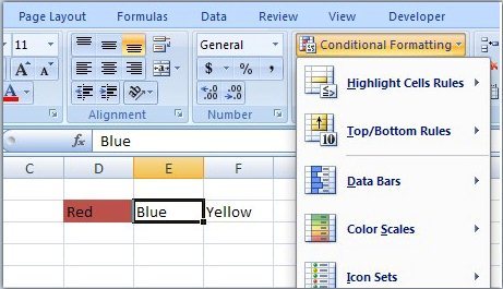
Conditional formatting is found in Home ribbon, in Styles.
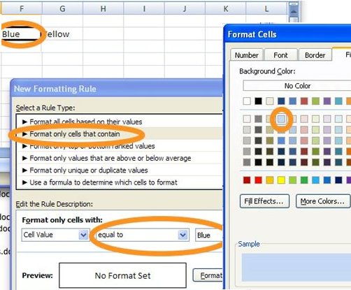
Highlight the cell(s) you want to work on then hit “New Rule”. This will allow you to set the condition you want the style to change based upon, and what you want the result to look like. So if, for example, we wanted the cell background colour to turn blue when the cell contains the word ‘Blue’, we could say “Format Only Cells That Contain”, “the Cell Value”, “Equal to”, “Blue”, then set the background fill to be a nice shade of blue.
It’s that easy!
More Complex Conditional Formatting
There are a lot of options when it comes to setting conditions. We can decide we want to have a certain formatting based on greater than, less than, a sliding scale or even a formula. We can either add the formula right into the cell rule or even have the formula depend on the outcome of a formula in the sheet!
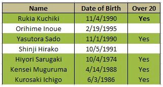
Let me explain using an example. Imagine we wanted to highlight rows in a table based on the age of the people represented. If they are over 20 we use one colour, under 20 we use another.
Do you see how the under-20s jump out of the screen?
First we discover if the person is over 20.
=IF(DATE(YEAR(TODAY())-20,MONTH(TODAY()),DAY(TODAY()))>=D5,"Yes","")
Then we set the conditional formatting formula to check if we have a ‘Yes’ in our E column.
Summary
Of course we have only scratched the surface of what conditional formatting can do, but I hope I have given you some inspiration so you can start using the feature in your own spreadsheets and maybe prevent some unnecessary data-induced headaches! Please let us know how you get on with your own.
About the author
This is a guest post by Yoav. Yoav Ezer co-authors the technology and productivity blog Codswallop. He is also the CEO of a company that produces PDF to Excel conversion software. Some previous articles by Yoav include Microsoft Excel alternatives, how to create lookup function in Google Docs, and How to protect cells in Excel.
For more Excel tips from Yoav, join him on Facebook or Twitter


